In many daily situations we can see parabolic motion, which is involving many factors such as gravity, velocity, acceleration, and time, where mathematics puts all in formulas explaining how it is formed and and continues (Lincoln, 2020). Two laws must be known in order to derive the parabolic trajectory of the motion, where one is the law of free fall and the other is restricted principle of inertia, as Galileo discovered the motion as a case of serendipity (Drake & MacLachlan, 1975). Two of features that are sometimes dicussed from the motion are maximum height and range (Boundless, 2018). There are animation showing the superposition of uniform and non-uniform linear motions (Henderson, 2022), calculator to find maximum height and range accompanied with their times (Had2Know, 2023), and interactive visualisation with adjustable parameters to show the influence of factors to the trajectory (Desmos, 2023). And it is also interesting that there is observation of perceptual judgments of duraction of parabolic motions in virtual reality world (Jörges et al., 2021). Sometimes it is assumed to be the same as free fall motion (Kumar, 2015), which is actually not (Albert, 2023). Here equation of trajectory, usually as y = f(x), is derived from two parametric equations representing uniform linear motion in x direction and non-uniform linear motion in y direction.
motion in x direction Link to heading
In horizontal direction, which is chosen as x direction, a point mass performs a uniform linear motion without acceleration or
$$ a_x = 0, $$
velocity
$$ v_x = v_{0x}, $$
and position
$$ x = x_0 + v_x t, $$
all at every time t, which is as
$$ x = x_0 + v_{0x} t, $$
usually written. Last equation is obtained by substituting the third last equation to the second last equation.
motion in y direction Link to heading
In vertical or y direction, it performs non-uniform linear motion since there is gravity which makes acceleration downward
$$ a_y = -g, $$
velocity
$$ v_y = v_{0y} - g, $$
and position
$$ y = y_0 + v_{0y}t - \tfrac12 gt^2, $$
which is similar to position in x direction, where the difference is the last term.
find expression for t Link to heading
Using one of previous equations time t can be expressed in the form of
$$ t = \frac{x - x_0}{v_{0x}}. $$
get function y = y(x) Link to heading
Substitute last this equation into position $y = y(t)$ will produce
$$ y = y_0 + \frac{v_{0y}}{v_{0x}} (x - x_0) - \frac{g}{2v_{0x}^2} (x - x_0)^2. $$
Previous equation can be rewritten as
$$ \begin{array}{rcl} y & = & \displaystyle \left( y_0 - \frac{v_{0y}}{v_{0x}} x_0 - \frac{g}{2v_{0x}^2} x_0^2 \right) \newline &&\newline && \displaystyle + \left( \frac{v_{0y}}{v_{0x}} + \frac{g}{v_{0x}^2} x_0 \right) x \newline &&\newline && \displaystyle + \left( - \frac{g}{2v_{0x}^2} \right) x^2, \end{array} $$
which shows the terms dependence on x to the power n-th. Or simply write it as
$$ y = c_0 + c_1 x + c_2 x^2, $$
with
$$ c_0 = \left( y_0 - \frac{v_{0y}}{v_{0x}} x_0 - \frac{g}{2v_{0x}^2} x_0^2 \right), $$
$$ c_1 = \left( \frac{v_{0y}}{v_{0x}} + \frac{g}{v_{0x}^2} x_0 \right), $$
and
$$ c_2 = \left( - \frac{g}{2v_{0x}^2} \right). $$
initial velocity and launch angle Link to heading
There are two ways to define initial velocity, where the first is using $v_{0x}$ and $v_{0y}$, which has been used in previous positions of $x$ and $y$. The second is using
$$ v_{0x} = v_0 \cos \theta $$
and
$$ v_{0y} = v_0 \sin \theta, $$
where v₀ is magnitude of initial velocity and θ is launch angle. The last two equations can be substitute to $c_0$, c₁, and c₂ to get
$$ y = y(x, v_0. \theta), $$
where the two last variables, v₀ and θ, can be considered as parameters since they value remain the same.
some graphs Link to heading
Using $y = y(x)$ some graphs can be drawn to show role of the parameters as follow.
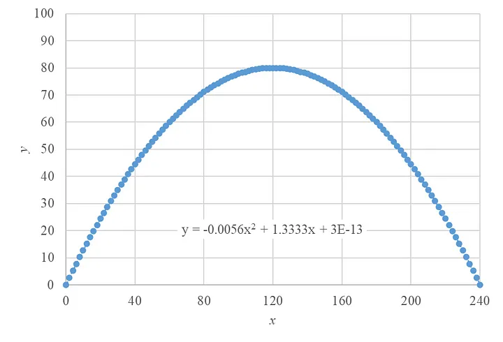
Above figure using following parameters tan θ = 4/3, v₀ = 50 m/s, x₀ = 0 m, y₀ = 0 m, which produce c₀ = 0 m, c₁ = 4/3 m⁻¹, and c₂ = — 5/900 m⁻². Unfortunately, Microsoft Excel Trendline does not give precise value of all c₀, c₁, and c₂. You can generate your own graph by modifying graphs.xlsx file.
Similar graph can also be produced using Python with Matplotlib, e.g. using following line of codes
import math
import matplotlib.pyplot as plt

# define environment constant
g = 10

# define initial conditions
x0 = 0
y0 = 0
theta = math.atan(4/3)
v0 = 50
v0x = v0 * math.cos(theta)
v0y = v0 * math.sin(theta)

# calculate coefficients
c0 = y0 - (v0y/v0x)*x0 - (g/2*v0x**2)*x0**2
c1 = (v0y/v0x) + (g/v0x**2)*x0
c2 = -(g/(2*v0x**2))
print("c0 =", c0)
print("c1 =", c1)
print("c2 =", c2)

# create data of x and y
N = 240
x = [*range(0, N+1)]
y = [(c0 + c1*i + c2*i**2) for i in x]

# plot data
plt.xlabel("x")
plt.xticks(range(0, 241, 60))
plt.xlim([0, 240])

plt.ylabel("y")
plt.ylim([0, 100])

plt.grid()

plt.plot(x, y, ".")
plt.show()
which can be modified online at https://trinket.io/python3/c152351717. Output on the console is as follow
c0 = 0.0
c1 = 1.3333333333333333
c2 = -0.005555555555555554
and the graph is below

which is similar to previous result.
challenges Link to heading
- Find the equation $y = y(x, v₀, θ)$. What would be the form of $y = y(x, x₀, y₀, v₀, θ)$? Is that the same as previous answer?
- How the maximum height can be obtained from $y = y(x, x₀, y₀, v₀, θ)$?
- How the range can be obtained from $y = y(x, x₀, y₀, v₀, θ)$?
- Shows that if $y(xₐ) = Hₐ$, the maximum height, then $xₐ — x₀ = 2R$, where $R$ is the range.
Read this on Medium @6unpnp/c484ff24fc79